P-values
Contents
P-values#
from datascience import *
from cs104 import *
import numpy as np
%matplotlib inline
1. Midterm Scores#
Was Lab Section 3 graded differently than that other lab sections, or could their low average score be attributed to the random chance of the students assigned to that section?
In this dataset, each row (observation) is a single student. There are 4 lab sections.
scores = Table().read_table("data/scores_by_section.csv")
scores.sample(5)
| Section | Midterm |
|---|---|
| 1 | 13 |
| 2 | 16 |
| 2 | 19 |
| 2 | 13 |
| 1 | 21 |
How many students in each section?
scores.group("Section")
| Section | count |
|---|---|
| 1 | 32 |
| 2 | 32 |
| 3 | 27 |
| 4 | 30 |
What was the mean Midterm score across each section?
scores.group("Section", np.mean)
| Section | Midterm mean |
|---|---|
| 1 | 15.5938 |
| 2 | 15.125 |
| 3 | 13.1852 |
| 4 | 14.7667 |
Lab section 3’s observed average score on the midterm.
observed_scores = scores.where("Section", 3).column("Midterm")
observed_scores
array([20, 10, 20,  8, 22,  0, 15, 23, 23, 18, 15,  9, 20, 10,  0, 10, 22,
       18,  4, 16,  7, 11, 11,  0, 16, 11, 17])
observed_average = np.mean(observed_scores)
observed_average
13.185185185185185
The observed sample size is the number of students in Lab Section 3.
observed_sample_size = scores.where("Section", 3).num_rows
observed_sample_size
27
Null hypothesis model: mean of the population
Null hypothesis restated: The mean in any sample should be close to the mean in the population (the whole class)
null_hypothesis_model_parameter = np.mean(scores.column("Midterm"))
null_hypothesis_model_parameter
14.727272727272727
Difference between Lab Section 3’s average midterm score and the average midterm score across all students.
observed_midterm_statistic = abs(observed_average - null_hypothesis_model_parameter)
observed_midterm_statistic
1.5420875420875415
Abstraction: Let’s create a function that calculates a statistic as the absolute difference between the mean of a sample and the mean of a population.
def statistic_abs_diff_means(sample):
    """Return the absolute difference in means between a sample and a population"""
    return np.abs(np.mean(sample) - null_hypothesis_model_parameter)
observed_midterm_statistic = statistic_abs_diff_means(observed_scores)
observed_midterm_statistic
1.5420875420875415
To simulate a sample from teh null hypothesis, we’ll sample without replacement to represent a different grouping of students into sections.
For example, these “could have been” Section 3 (if it was sample size 5).
sample = scores.sample(5, with_replacement=False)
sample
| Section | Midterm |
|---|---|
| 1 | 21 |
| 4 | 15 |
| 1 | 20 |
| 3 | 17 |
| 4 | 21 |
sample.column("Midterm")
array([21, 15, 20, 17, 21])
Let’s put this into a function we can later put into simulate_sample_statistic.
def sample_scores(sample_size):
    """
    Sampling scores with replacement

    Note: we're using with_replacement=False here because we don't
    want to sample the same student's score twice.
    """
    return scores.sample(sample_size, with_replacement=False).column("Midterm")
sample_scores(observed_sample_size)
array([10, 14, 11, 11,  7,  7, 14, 14, 13, 13, 24, 23, 15, 13, 10, 10, 21,
       13, 13, 20,  0, 14,  9, 14, 18, 23, 20])
simulated_midterm_statistics = simulate_sample_statistic(sample_scores,
                                         observed_sample_size,
                                         statistic_abs_diff_means,
                                         5000)
results = Table().with_columns("Statistic: abs(sample mean - population mean)",
simulated_midterm_statistics)
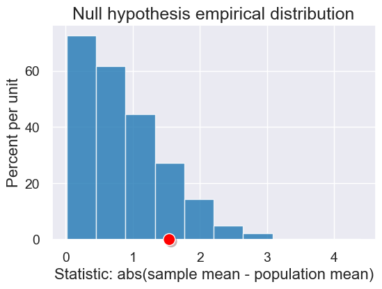
plot = results.hist(title="Null hypothesis empirical distribution")
plot.dot(observed_midterm_statistic)
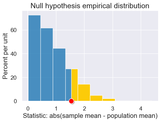
2. Calculating p-values#
def plot_simulated_and_observed_statistics(simulated_statistics, observed_statistic):
    """
    Plots the empirical distribution of the simulated statistics, along with
    the observed data's statistic, highlighting the tail in yellow.
    """
    results = Table().with_columns("Statistic: abs(sample mean - population mean)",
                                   simulated_statistics)
    plot = results.hist(left_end=observed_statistic, title="Null hypothesis empirical distribution")
    plot.dot(observed_statistic)
plot_simulated_and_observed_statistics(simulated_midterm_statistics, observed_midterm_statistic)
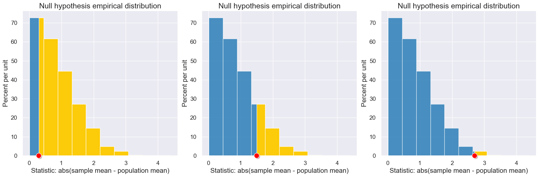
Supposed we observed other observed statistics: 0.3, 1.5, and 2.7:
with Figure(1,3):
    plot_simulated_and_observed_statistics(simulated_midterm_statistics, 0.3)
    plot_simulated_and_observed_statistics(simulated_midterm_statistics, 1.5)
    plot_simulated_and_observed_statistics(simulated_midterm_statistics, 2.7)
Calculating p-values: Let’s compute the proportion of the histogram that is colored yellow. This captures the proportion of the simulated samples under the null hypothesis that are more unlikely than the observed data.
We’ll do it first for our midterm example, and then generalize to a function we can use to compute p-values for any test.
simulated_midterm_statistics
array([0.54208754, 1.12457912, 1.75420875, ..., 1.34680135, 1.06060606,
       1.20875421])
np.count_nonzero(simulated_midterm_statistics >= observed_midterm_statistic) / len(simulated_midterm_statistics)
0.1526
Now as a function:
def empirical_pvalue(null_statistics, observed_statistic):
    """
    Return the proportion of the null statistics that are greater than
    or equal to the observed statistic.
    """
    return np.count_nonzero(null_statistics >= observed_statistic) / len(null_statistics)
empirical_pvalue(simulated_midterm_statistics, observed_midterm_statistic)
0.1526
3. Impact of Sample Size on p-value#
Recall that as our sample size increases, we observe less variability in our samples.
Here’s a visualizaion showing the Null hypothesis empirical distribution for different sample sizes. Note how the p-value changes as the sample size changes due to that effect.
def visualize_p_value_and_sample_size(sample_size):

    simulated_midterm_statistics = simulate_sample_statistic(sample_scores,
                                         sample_size,
                                         statistic_abs_diff_means,
                                         1000)

    results = Table().with_columns("Statistic: abs(sample mean - class mean)",
                                   simulated_midterm_statistics)
    plot = results.hist(left_end=observed_midterm_statistic,bins=np.arange(0,6,0.2))

    plot.dot(observed_midterm_statistic)
    plot.set_ylim(0,2)

    pvalue = empirical_pvalue(simulated_midterm_statistics, observed_midterm_statistic)
    plot.set_title('sample-size = ' + str(sample_size) + '\np-value = '+str(pvalue))


interact(visualize_p_value_and_sample_size,
         sample_size=Slider(5,80))
Here’s the same visualization as an animation.