Hypothesis Testing#

from datascience import *
from cs104 import *
import numpy as np
%matplotlib inline

1. Single category null hypothesis test: Swain v. Alabama#

Here is the basic setup for our Swain jury panel example.

# Population
population_percent_black = 26
population_proportions = make_array(population_percent_black / 100,
                                    1 - population_percent_black / 100)

# Observed Sample
swain_percent_black = 8
swain_proportions = make_array(swain_percent_black / 100, 
                               1 - swain_percent_black / 100)

We’ll now set up our simulation in terms of a null hypothesis and alternate hypothesis, as well as a statistic measure how close an observed panel is to what is predicted under the null hypothesis:

Null hypothesis: Each panelist is drawn randomly from the population. So, Chance each panelist is black is 26%.
Alt. hypothesis: Each panelist is not drawn randomly from the population. So, Change each panelist is black is not 26%.
Sample statistic: Given a sample, compute abs(percent black - 26).

Simulating under the null hypothesis#

Same as before, we’ll simulate a sample for a single category (percent black), with sample_proportions.

def simulate_panel_sample(sample_size):
    """Return an array with the counts of [black, non-black] panelists in sample."""
    props = sample_proportions(sample_size, population_proportions)
    return np.round(sample_size * props)  # no fractional persons

Sample Statistic#

We will only look at two-sided hypothesis tests. This means we don’t care about the whether a value is greater or less than the null hypothesis but just if it’s different so we will use absolute values here.

def statistic_abs_difference(sample): 
    """ Absolute difference between: 
    - Percent black panelists (for any sample size)
    - Null hypothesis of 26 
    """
    percent_black = sample.item(0) / sum(sample) * 100
    return abs(percent_black - population_percent_black)

Run the simulation#

all_outcomes = simulate_sample_statistic(simulate_panel_sample, 100, 
                                         statistic_abs_difference, 5000) 

simulated_results = Table().with_column('abs(percent black - 26)', 
                                        all_outcomes)
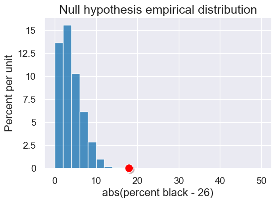
plot =simulated_results.hist(bins=np.arange(0, 51, 2))
plot.set_title("Null hypothesis empirical distribution")

# Red dot for the statistic on the observed (not simulated) data
observed_stat = statistic_abs_difference(swain_proportions)
plot.dot(observed_stat)

../_images/20-hypothesis-testing_15_0.png

So, clearly, the observed panel is not concistent with what we would expect under the null hypothesis.

Impact of sample size#

Sample size has a large impact on the results of our simulation. Here are three scenarios in which we vary the size of the jury panels. In each, suppose we observe a jury panel that is 15% black:

../_images/20-hypothesis-testing_20_0.png

Notice that with small samples of 20, we cannot say that a 15% black panel is inconsistent with the null hypothesis. With samples of 100, we do see some panels with 15% or less, so again, it is hard to say anything conclusively. With samples of 1,000, we don’t see any, and it is very easy to conclude that our observed panel is inconsistent with the null hypothesis. In general, the larger the sample, the less smaller the variability in our statistic.

Here is an interactive visualization of that effect:

sample_size

swain_percent_black

In the next lecture, we’ll introduce a technique to say something better about the middle case where it isn’t obvious.

2. Multiple category null hypothesis test: Alameda, California Jury Panels#

Null hypothesis: Each panelist is drawn randomly from the population. So, Ethnicity distribution of a panel is the same as distribution of the population.
Alt. hypothesis: Each panelist is not drawn randomly from the population. So, Ethnicity distribution of a panel not the same as the distribution of the population.
Sample statistic: TVD from ethnicity distribution for population.

Let’s first load the data from the ACLU study. Here is the ethnicity distrubtion of the whole population of eligible voters and of the observed panels.

jury = Table().with_columns(
    'Ethnicity', make_array('Asian/PI', 'Black/AA', 'Caucasian', 'Hispanic', 'Other'),
    'Population (Eligible)', make_array(0.15, 0.18, 0.54, 0.12, 0.01),
    'Observed (Panels)', make_array(0.26, 0.08, 0.54, 0.08, 0.04)
)

jury

Ethnicity	Population (Eligible)	Observed (Panels)
Asian/PI	0.15	0.26
Black/AA	0.18	0.08
Caucasian	0.54	0.54
Hispanic	0.12	0.08
Other	0.01	0.04

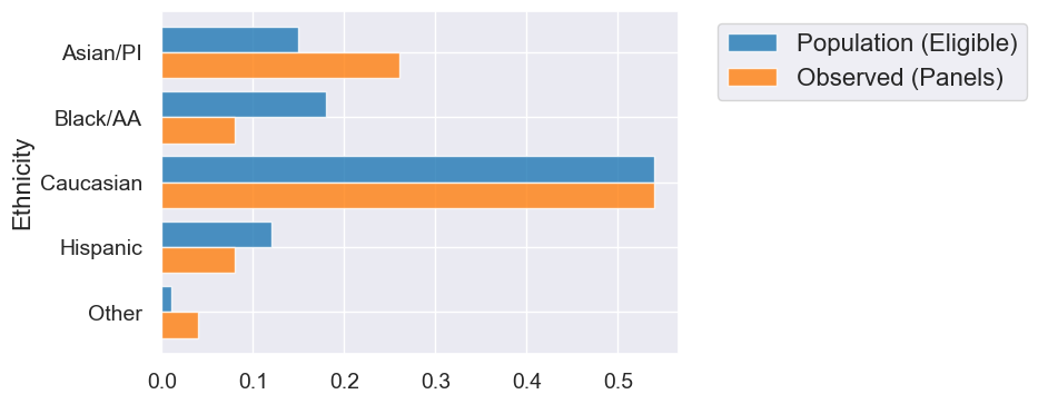
Let’s create an overlaid bar chart to compare the population and observed distributions across ethnicity.

jury.barh('Ethnicity')

../_images/20-hypothesis-testing_31_0.png

We can use sample_proportions with distributions with multiple categories as well.

distribution = make_array(0.1, 0.2, 0.7)
sample_proportions(10, distribution)

array([0.1, 0.2, 0.7])

Sample#

To create a sample for the null hypothesis, we’ll use sample_proportions on the true distribution of ethnicities in the population.

def simulate_sample_alameda(sample_size):
    """
    Sample from the eligible population 
    """
    eligible_population = jury.column('Population (Eligible)')
    return sample_proportions(sample_size, eligible_population)

study_size = 1453
simulated_sample = simulate_sample_alameda(study_size)
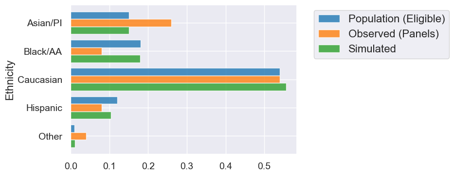
jury_with_simulated = jury.with_columns("Simulated", simulated_sample)
jury_with_simulated.barh("Ethnicity")

../_images/20-hypothesis-testing_37_0.png

TVD Statistic: Distance Between Two Distributions#

jury.barh('Ethnicity')

../_images/20-hypothesis-testing_39_0.png

jury_with_diffs = jury.with_columns(
    'Difference', jury.column('Observed (Panels)') - jury.column('Population (Eligible)')
)
jury_with_diffs

Ethnicity	Population (Eligible)	Observed (Panels)	Difference
Asian/PI	0.15	0.26	0.11
Black/AA	0.18	0.08	-0.1
Caucasian	0.54	0.54	0
Hispanic	0.12	0.08	-0.04
Other	0.01	0.04	0.03

jury_with_diffs = jury_with_diffs.with_columns(
    'Absolute Difference', np.abs(jury_with_diffs.column('Difference'))
)

jury_with_diffs

Ethnicity	Population (Eligible)	Observed (Panels)	Difference	Absolute Difference
Asian/PI	0.15	0.26	0.11	0.11
Black/AA	0.18	0.08	-0.1	0.1
Caucasian	0.54	0.54	0	0
Hispanic	0.12	0.08	-0.04	0.04
Other	0.01	0.04	0.03	0.03

sum(jury_with_diffs.column('Absolute Difference') / 2)

0.14

Here it is all at once.

def total_variation_distance(distribution1, distribution2):
    return sum(np.abs(distribution1 - distribution2)) / 2

observed_panels = jury.column('Observed (Panels)')
eligible_population = jury.column('Population (Eligible)')
total_variation_distance(observed_panels, eligible_population)

0.14

A combined sample and statistic computation. Run it a bunch!

simulated_sample = simulate_sample_alameda(study_size)
total_variation_distance(simulated_sample, eligible_population)

0.025251204404680008

Our simulated_sample_statistic function expects our compute_one_statistic function that to have just a single argument, namely the sample. In this case, that sample would be a simulated panel.

def tvd_from_population(sample_panel): 
    return total_variation_distance(sample_panel, eligible_population)

tvd_from_population(simulated_sample)

0.025251204404680008

All together: Simulating under the null#

all_outcomes = simulate_sample_statistic(simulate_sample_alameda, 1453, 
                                         tvd_from_population, 5000)

simulated_tvds = Table().with_column('TVD from eligible population', 
                                     all_outcomes)

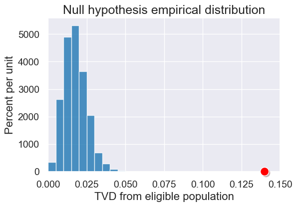
plot = simulated_tvds.hist(bins=np.arange(0, 0.2, 0.005))

# Create the observed statistic 
observed_panels = jury.column('Observed (Panels)')
observed_statistic = tvd_from_population(observed_panels)
plot.dot(observed_statistic)

plot.set_title('Null hypothesis empirical distribution')
plot.set_xlim(0, 0.15)

../_images/20-hypothesis-testing_53_0.png

CSCI 104: Data Science and Computing for All

Hypothesis Testing

Contents